We define a dynamic correlation function as
(1)
where  and
and  are operators.
Since pi-qmc uses a position basis, we often collect density fluctuations in real space. However, most textbook descriptions of density fluctioans are in k-space, and results for homogeneous systems are often best represented in k-space. Here we give a brief summary of common definitions for pedagogical purposes. For simplicity we write all formulas for spinless particles.
The dimensionsless Fourier transform of the density operator is (Eqs. 1.11 and 1.66 of Giuliani and Vignale)
(2)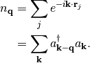
Note that  ,
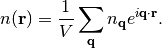
the total number of particles. To get back to real-space density use
,
the total number of particles. To get back to real-space density use
(3)
For each of these, we define frequency-dependent density operators,
(4)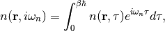
and
(5)
where  are the Matsubara frequencies. Within the pi-qmc code, these
frequency-dependent densities are easily calculated with fast Fourier
transforms, which are most efficient when the number of slices is a power of
two.
are the Matsubara frequencies. Within the pi-qmc code, these
frequency-dependent densities are easily calculated with fast Fourier
transforms, which are most efficient when the number of slices is a power of
two.
The imaginary-frequency response of the density to an external perturbation is given by (Ch 3.3 of Guiliani and Vignale),
(6)
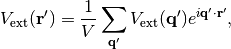
In k-space this takes the convienent form,
(7)
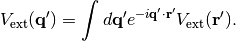
where the external potential in k-space satisfies
(8)
and
(9)
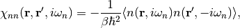
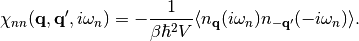
These response functions are related to imaginary-frequency dynamic correlation functions,
(10)
and
(11)
For a homogeneous system,
(12)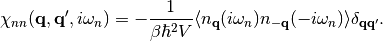
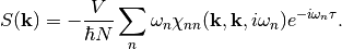
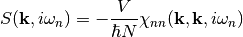
The dynamic structure factor S(k,iωn) measures the density response of the system,
(13)
The static structure factor is defined for equal time, not for
 ,
,
(14)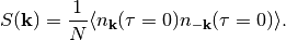
In terms of 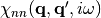 ,
the static structure factor is given by (prefactor is wrong)
,
the static structure factor is given by (prefactor is wrong)
(15)