![]()
Table Of Contents
Previous topic
Actions: Describing the Dynamics
Next topic
Algorithms: Describing the Sampling Strategy
![]()
Actions: Describing the Dynamics
Algorithms: Describing the Sampling Strategy
The simplest way to collect the density is to create a rectangular array of bins and histogram the beads of the paths. For example, a grid defined by
has nx*ny*nz rectangular bins, each with dimension dx = (xmax-xmin)/nx by dy = (ymax-ymin)/nz by dz = (zmax-zmin)/nz. The bin with indicies (i, j, k) is centered at ( xmin+(i+0.5)*dx, ymin+(j+0.5)*dy, zmin+(k+0.5)*dz ).
Each time a measurement is made, the position of all npart*nslice beads is checked, where npart is the number of particles of the species whose density is being measured. If a bead is inside one of the bins, that bin is increased by 1./nslice. If all beads lie in the grid bins, then the bins sum to npart. Otherwise the total is less than npart; this can happen if the grid dimensions do not fill the simulation supercell. To convert the measurement to density, divide by the volume of a bin, dx * dy * dz.
<DensityEstimator>
  <Cartesian dir="x" nbin="500" min="-250 nm" max="250 nm"/>
  <Cartesian dir="y" nbin="500" min="-255 nm" max="250 nm"/>
</DensityEstimator>
Since pi-qmc uses a position basis, we often collect density fluctuations in real space. However, most textbook descriptions of density fluctioans are in k-space, and results for homogeneous systems are often best represented in k-space. Here we give a brief summary of common definitions for pedagogical purposes. For simplicity we write all formulas for spinless particles.
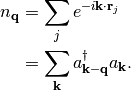
The dimensionsless Fourier transform of the density operator is (Eqs. 1.11 and 1.66 of Giuliani and Vignale)
(1)
Note that  , the total number of particles.
The pi code does not presently calculate this expectation value. If it is implemented in the future, it should return a complex expectation value for each k-vector. The imaginary part of this estimator will be zero for systems with inversion symmetry about the origin.
Homegeneous systems, such as liquid helium or the electron gas, will have
 for all
  .
In those cases, it is better to calculate the
static structure factor
(see static structure factor).
.
In those cases, it is better to calculate the
static structure factor
(see static structure factor).
We define a dynamic correlation function as
(2)
where  and
and  are operators.
Since pi-qmc uses a position basis, we often collect density fluctuations in real space. However, most textbook descriptions of density fluctioans are in k-space, and results for homogeneous systems are often best represented in k-space. Here we give a brief summary of common definitions for pedagogical purposes. For simplicity we write all formulas for spinless particles.
The dimensionsless Fourier transform of the density operator is (Eqs. 1.11 and 1.66 of Giuliani and Vignale)
(3)
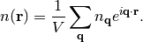
Note that  ,
the total number of particles. To get back to real-space density use
,
the total number of particles. To get back to real-space density use
(4)
For each of these, we define frequency-dependent density operators,
(5)
and
(6)
where  are the Matsubara frequencies. Within the pi-qmc code, these
frequency-dependent densities are easily calculated with fast Fourier
transforms, which are most efficient when the number of slices is a power of
two.
are the Matsubara frequencies. Within the pi-qmc code, these
frequency-dependent densities are easily calculated with fast Fourier
transforms, which are most efficient when the number of slices is a power of
two.
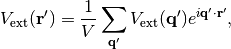
The imaginary-frequency response of the density to an external perturbation is given by (Ch 3.3 of Guiliani and Vignale),
(7)
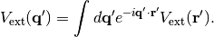
In k-space this takes the convienent form,
(8)
where the external potential in k-space satisfies
(9)
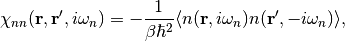
and
(10)
These response functions are related to imaginary-frequency dynamic correlation functions,
(11)
and
(12)
For a homogeneous system,
(13)
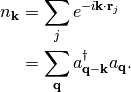
The dynamic structure factor S(k,iωn) measures the density response of the system,
(14)
The static structure factor is defined for equal time, not for
 ,
,
(15)
In terms of  ,
the static structure factor is given by (prefactor is wrong)
,
the static structure factor is given by (prefactor is wrong)
(16)