Introduction: Quantum Simple Harmonic Oscillator
Pi-qmc is a computer program in the language of C++ that predicts the behavior of quantum, or atomically small, particles. These particles do not always behave in the same manner as larger bodies and must be studied using unique equations. Quantum particles behave more and more like larger bodies as their energy increases.
Pi-qmc is able to easily predict the motion of these particles by summing the potential motions found using a random walk where the motions are predicted using statistical equations. Normally, the behavior of quantum systems would have to be found using a far more difficult process where the energies of each eigenstate are summed and divided by the number of possible states in order to normalize the function and find the average energy. A simple example of a quantum system where this process could be applied is the Quantum Harmonic Oscillator (QHC). The mathematics behind this process start with calculating the total energy of the system.
Background
The total energy, or Hamiltonian, of a Quantum Harmonic Oscillator is represented by the function
(1)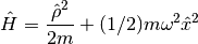
The kinetic energy of the quantum harmonic oscillator is represented by the first term while the stored energy is represented by the second term. This may seem complex at first glance, but upon further inspection, it becomes apparent that this Hamiltonian is nearly identical to Hamiltonian of a regular harmonic oscillator which is represented by the function
(2)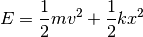
In the Hamiltonian of a Quantum Harmonic Oscillator, the mass multiplied by the velocity can be substituted in place of the momentum and the first term can be rearranged to resemble the first term of the regular harmonic oscillator’s Hamiltonian. Similarly, the square root of the spring constant divided by the mass can be substituted in for the wavelength and the second term can be rearranged to resemble the second term of the regular harmonic oscillator. After both terms are rearranged, it becomes clear that the two Hamiltonians are identical.
Eigenstates of the Simple Harmonic Oscillator
The Eigenstate of Quantum Harmonic Oscillator is the energy level it occupies. These energy levels are represented by whole numbers (n=0, n=1, n=2, …) and are separated by consistent amounts energy that increase with each consecutive energy level. As the eigenstate increases, the period of the quantum harmonic oscillator decreases and the wave behaves differently. The energy of the eigenstate, or eigenvalue can be found using the function
(3)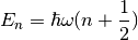
According to Heisenberg’s Uncertainty Principle, the momentum and the position of a quantum particle cannot be known at the same time. Therefore, we can surmise that the energy of the eigenvalue will never be equal to zero since the no energy means no movement which, in turn, means that both the momentum and the position of the quantum particle will be known. When we substitute in a 0 for the eigenvalue, we find that the function simplifies to
(4)
which represents the lowest possible energy of the Eigenstate and agrees with Heisenberg’s Uncertainty principle.
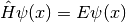
When the eigenstate is multiplied by the Hamiltonian, the resulting value is the eigenvalue as shown in the function
(5)
The Classical Partition Function
The Quantum Mechanical Partition Function
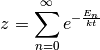
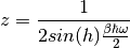
In one dimension, the partition function of the simple harmonic oscillator is
(6)![Z = \sum_{n=0}^\infty e^{-\beta\hbar\omega (n+\frac{1}{2})}
= \left[2\sinh\left(\frac{\hbar\omega}{2k_BT}\right)\right]^{-1}](_images/math/a9a1569a413c8232b5bdf4984d143b7f95b069cb.png)
For N oscillators in D dimensions, the partition function is
(7)![Z = \left[2\sinh\left(\frac{\hbar\omega}{2k_BT}\right)\right]^{-ND}](_images/math/2346df7b5134ae14c8c630acd6c1eae6befe254a.png)
The Helmholtz free energy is
(8)![F = E - TS = -k_BT \ln(Z)
= ND k_BT \ln\left[2 \sinh\left(\frac{\hbar\omega}{2k_BT}\right)\right].](_images/math/05eccad1eb1c9270f051dbbb8de42413f6c58ebd.png)
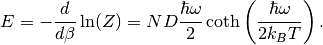
The total energy is
(9)
Normalizing the Function
The function is now normalized by dividing by the partition function
(10)
This function can be simplified to the form
(11)
where
(12)
Our final equation is now
(13)
The Density Matrix
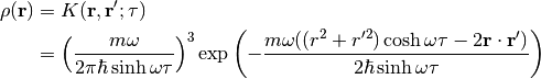
For one particle in a haromonic confinining potential
in three dimensions, the imaginary time propagator is
(14)
The diagonal of the density matrix is the probability density,
(15)
Simulating a Simple Harmonic Oscillator
Calculating the Energy
Calculating the Density
Calculating the Polarizability
 (line 5),
and we are simulating a harmonic oscillator with
(line 5),
and we are simulating a harmonic oscillator with  Hartrees (line 8).
From Eq.
Hartrees (line 8).
From Eq.  .
.